| Issue |
Sust. Build.
Volume 8, 2025
|
|
|---|---|---|
| Article Number | 2 | |
| Number of page(s) | 12 | |
| Section | Modelling and Optimisation of Building Performance | |
| DOI | https://doi.org/10.1051/sbuild/2025002 | |
| Published online | 18 July 2025 | |
Original Article
Wind resistance performance optimization of PSO algorithm in skyscrapers design
School of Architecture and Engineering, Lianyungang Technical College, Lianyungang, 222000, China
* e-mail: This email address is being protected from spambots. You need JavaScript enabled to view it.
Received:
28
September
2024
Accepted:
10
June
2025
Abstract
To optimize the skyscrapers and enhance its wind resistance performance under wind load, a wind resistance optimization method for super high-rise building structure on the basis of improved Particle Swarm Optimization (PSO) is built. Through the harmonic excitation method, the equivalent static wind load is calculated, and the desired mathematical model is constructed. The chaotic mapping technology is introduced and the chaotic local search strategy is adopted to further accurately optimize the update process of the global optimal solution. The PSO converged rapidly in the first 50 iterations. The objective function value decreased from about 0.45 to less than 0.1, and then the decline rate slowed down and tended to be stable. After 150 iterations, it was basically stable and close to 0, indicating that the optimal solution was found. The initial target value of quantum-behaved PSO was about 0.5, which decreased rapidly in the first 50 times, and slowly optimized from 50 to 200 times, and then tended to be stable and close to 0 after 200 times. The algorithm converged rapidly in the first 50 times, and had good stability after 200 times, which could find a better solution. The displacement and stress of the optimized structure under wind load meet the specification, the local search efficiency of quantum-behaved PSO is higher, and the global search ability is enhanced by chaotic mapping.
Key words: QPSO / logistic / skyscrapers / large-span roof / wind resistance
© S. Wang, Published by EDP Sciences, 2025
 This is an Open Access article distributed under the terms of the Creative Commons Attribution License (https://creativecommons.org/licenses/by/4.0), which permits unrestricted use, distribution, and reproduction in any medium, provided the original work is properly cited.
1 Introduction
Skyscrapers are buildings with more than 40 floors or more than 100 meters in height. In recent years, skyscrapers have developed rapidly [1]. As the main natural disaster affecting human activities, wind disaster has a significant impact on the upper floors of skyscrapers. Due to the lack of shelter, the upper floor is subject to strong wind load, which leads to significant vibration and brings discomfort and panic to people. Super high-rise buildings have complex structures, numerous components, and diverse stress conditions. The traditional design method is time-consuming, laborious, and conservative [2,3]. However, strengthening the building structure to resist the wind load is not only expensive, but also increases the building weight. Reducing acceleration response under wind load and improving comfort have always been the research focus of engineers. Ensuring the structural safety of skyscrapers is currently a key focus [4]. Kumar and Prakash analyzed the application of micro wind turbines in high-rise buildings and used them as turbine towers. Based on the wind chart, the wind behavior at different heights was analyzed, and the wind power generation potential of different states in India was evaluated. The results showed that the micro wind turbine also performed well in the home [5]. Wang and Zhang analyzed the wind load distribution, Equivalent Static Wind Load (ESWL) and wind-induced response of skyscrapers. The maximum values of wind-induced overturning moment and acceleration response occurred in 60° and 330° wind directions. The aerodynamic interference of surrounding buildings affected the wind pressure distribution [6]. To enhance the stability of skyscraper steel structures, Lu et al. calculated the additional internal force on the basis of the stress model. The node data was divided into terrain and ground object data. The noise was reduced by filtering, and the laser scanning data was processed. Combined with these data, the wind-induced reliability was analyzed using the stiffness formula, demonstrating high reliability and short analysis time [7]. Cui et al. measured the surface pressure of three skyscrapers through wind tunnel test. The influence of various wind direction angles and spacing ratios on shape coefficient was analyzed. The fluctuation of wind pressure coefficient was influenced by the spacing ratio [8].
The long-span roof structure refers to the roof structure covering a large area of space and with a long span. Its structural stability and wind resistance performance need to be specially considered in the design and optimization process [9]. Chen et al. used nonlinear dynamic time history analysis to study the wind-induced response characteristics of the structure. With the increase of wind speed, the maximum displacement shifted from the top to the windward area, which may lead to displacement overrun [10]. Air rib tents are popular for their portability and adaptability, but their large deformation reduces the effective space, and parameter optimization can reduce the displacement. Liu et al. discussed the influence of external factors on the tent. The angle and number of wind ropes had the greatest influence on the displacement. Based on the response surface method, the obtained wind rope angle was 41°, and the initial prestress of the end wind rope was 800Pa. After optimization, the maximum displacement decreased by 10.2%, and the maximum stress changed little [11]. Wang et al. constructed a large-span integral tension structure of ETFE roof based on two-way cable net support. The construction project ensured the structural stability, shortened the construction period and reduced the cost. The prestress level was the key step of flexible structure design optimization. The whole process required high precision and high standard [12]. Chen et al. analyzed the long-span transversely reinforced suspension cable system considering the construction period. The Newton-Raphson method was applied for geometric nonlinear analysis. The maximum shape error was between 0.33% and 0.98%, and the shape control was accurate. The load response analysis showed that the strength criterion mainly controlled the stress level, and the stiffness criterion controlled the shape, realizing the accurate control of the shape in the self balanced state [13].
To sum up, some research focus on the wind-induced response of a specific wind direction and a single building, but lack comprehensive research on multiple buildings, and fail to fully consider the wind load characteristics under different terrain and climate. When simulating super high-rise buildings, some studies ignore the nonlinear characteristics of the detail structure and materials, resulting in the deviation between the results and the actual situation. There are errors in stress model and finite element analysis when dealing with complex wind loads, especially in high wind speed and extreme conditions. Quantum-behaved Particle Swarm Optimization (QPSO) has global search ability, fast convergence speed and strong adaptability. It has a wide application in optimizing wind resistance performance when designing skyscrapers. Therefore, the chaotic mapping is introduced to improve the local optimization of QPSO. A wind resistant optimization model is built to minimize the sectional area of the member and satisfy the constraints of displacement and stress. The optimal design scheme is selected using the sum of particle distance and penalty function. The research aims to further optimize the wind resistance performance and design efficiency of skyscrapers by combining the improved PSO algorithm with the existing wind tunnel test methods.
2 Methods and materials
The improved QPSO combines wind tunnel test data and numerical simulation methods to optimize the wind resistance performance of skyscrapers and large-span roof structures. Firstly, the ESWL is calculated by harmonic excitation method and Load Response Correlation (LRC) method, and the wind resistance optimization mathematical model satisfying the displacement and stress constraints is established. To improve the convergence effect of QPSO, chaos mapping technology introduced, which is an optimization method based on chaos theory. Chaotic variables are introduced to replace random variables in the traditional algorithm to enhance the global search ability and convergence speed. Chaotic maps are deterministic and pseudo-random, which can explore the search space more evenly in the global range, and avoid falling into local optimal solution.
2.1 Wind resistant design of skyscrapers structures based on QPSO
Wind tunnel test technology is used to simulate and analyze the effect of air flow on objects. By placing a reduced scale model in the wind tunnel, the wind speed and direction are controlled, and the force and pressure distribution caused by air flow are analyzed to help evaluate the wind resistance performance, aerodynamic characteristics and wind load distribution of the structure. The wind load calculation process usually includes the following steps. First, determine the basic wind speed, wind direction frequency, surface roughness and other meteorological parameters of the building location. Then, depending on the basic wind speed, the wind pressure is calculated, usually using the standard formula. Then, considering the shape and structural characteristics of buildings, wind pressure distribution, especially for high-rise buildings and long-span structures, height changes and local effects should be considered. After that, the wind pressure is converted into ESWL and distributed in key parts. The wind load is used to analyze the structure, check the displacement, stress and other responses, and optimize the design according to the results. The test wind direction angle and measuring point arrangement are shown in Figure 1.
In Figure 1, the pressure measurement test design covers seven different wind directions, ranging from 90° to 180°, and the measurement is made every 15°. Through this fine arrangement, the pressure distribution characteristics of each wind direction can be fully captured, which provides detailed data support for the wind resistance performance analysis of the structure. Harmonic Excitation Method (HEM) is a technology used to examine the dynamic response of structures. It simulates the periodic external excitation of structures in the actual environment by applying harmonic excitation of a specific frequency [14,15]. Due to the large degree of freedom of long-span structures, HEM can improve the calculation efficiency while ensuring the accuracy, as displayed in formula (1).
 (1)
(1)
In formula (1), [M], [C] and [K] signify mass matrix, damping matrix, and stiffness matrix. The dimensions of the three matrices are n × n. {y},  and
and  represent displacement vector, velocity vector, and acceleration vector. The dimensions of the three vectors are n × 1. The random load vector is denoted as {pT (t)}. The truncated function vector is constructed by p (t). The research on equivalent wind load mainly includes gust load factor method, inertial wind load method and LRC [16]. The ESWL of long-span roof structure under wind vibration is calculated by LRC method. The ESWL is shown in formula (2).
 (2)
(2)
In formula (2),  represents the average wind load matrix, representing the average wind load on each degree of freedom, with a dimension n × nr. gf is the gust factor, a scalar, which is used to adjust the wind load to consider the gust effect. ρrf stands for the load correlation matrix, and the dimension is n × nr, indicating the correlation of wind loads between different degrees of freedom. T represents the transpose symbol of the matrix, which means to transpose the matrix
  . σf signifies the standard deviation matrix of wind load, with dimension n × nr, representing the standard deviation in each degree of freedom, which is applied to quantify the fluctuation of wind load. The wind resistance optimization model is shown in formula (3) [17].
 (3)
(3)
In formula (3), minf (x) represents the wind resistance of the entire system or some energy consumption indicator related to it. ρ represents the weight coefficient related to wind resistance. xi represents the ith optimization variable. li represents the coefficient of the ith optimization variable. v (x) represents the wind speed under the system design result. [v] is the allowable upper limit of wind speed. σ (x) represents the stress or response value of a physical quantity under the design result of the system. [σ] represents the allowable upper limit corresponding to σ (x).  and
and  represent the upper and lower limits of the j th design variable, respectively. The construction of wind resistance optimization model is the core to improve the wind resistance performance of skyscrapers. In this process, PSO algorithm will play a key role in finding the optimal solution in structural design by simulating the flight behavior of particle swarm. This involves not only the determination of the geometry and material parameters of the structure, but also the minimization of the cross-sectional area of the member under the premise of satisfying the displacement and stress constraints. In this way, it is possible to optimize the use of materials and reduce construction costs while ensuring the safety of the structure. The QPSO algorithm introduces the concept of quantum dynamics on the ground of the original PSO, eliminating the velocity and direction of particle movement. It can more effectively solve high-dimensional and complex optimization problems. The wind resistance optimization process of skyscrapers structures on the basis of QPSO is displayed in Figure 2.
In Figure 2, first, the problem is encoded and the QPSO is initialized, including population size and maximum iterations. After initialization, the generated solution is subjected to feasibility testing. If the solution is not feasible, it is adjusted through mutation operations to ensure that it meets the constraint conditions. Next, the fitness of each feasible solution is calculated based on indicators such as structural weight, displacement and stress under wind loads. Afterwards, the Individual Optimal Solution (Pbest) is calculated, and the Global Optimal Solution (Gbest) of the population is determined. By updating the velocity and position, they can explore better solutions. The iterative process continues until the predetermined stopping condition or maximum iterations are satisfied, and the final output is the optimal solution. This process provides diversity of initial solutions for subsequent optimization calculations, ensuring that the algorithm can effectively explore the Gbest. The cross-sectional area of steel structure circular pipes is shown in formula (4).
 (4)
(4)
In formula (4), xi,j signifies the value of the j-th variable in the i-th design scheme, indicating the specific area of the steel structure circular pipe section under the current scheme.  represents the lower limit value of the j-th variable, which is the minimum allowable value of the cross-sectional area of the steel structure circular tube.
  represents the upper limit value of the j-th variable, which is the maximum allowable cross-sectional area of the steel structure circular tube. ϵ signifies a random number equally distributed [0,1] to generate random variable values between the lower and upper limits. The displacement and stress response under equivalent wind load are determined through structural analysis to obtain the constraint redundancy. The fitness values of each scheme are evaluated to select the best design. Compared with the previous generation's optimal solution, the Gbest is updated. According to the QPSO algorithm, the next generation design scheme is updated. If the particle exceeds the feasible region, the sectional area of the member is adjusted and pulled back into the feasible region using formula (5).
 (5)
(5)
If it is detected that the design scheme does not meet these key indicators, it is necessary to return for re-evaluation and optimization of structural design parameters, which may include adjusting the parameter settings of the QPSO algorithm or the initial conditions during the optimization process. Through continuous iteration and verification, the selected solution is ultimately ensured to achieve the best balance in terms of structural weight, wind resistance, and material utilization, meeting the strict requirements of the design specifications. If not, the total weight of the structure is recalculated. Afterwards, by changing the parameters of the QPSO algorithm and repeating the optimization process, the impact of each parameter on wind resistance optimization is analyzed.
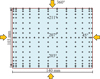 |
Fig. 1 Definition of test wind direction and arrangement of measuring points. |
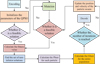 |
Fig. 2 Wind resistance optimization process of super tall building structure based on QPSO algorithm. |
2.2 Wind resistant optimization design of large-span roof structures based on chaotic mapping
QPSO can decide the geometric model and material parameters of large-span roof structures in wind resistant design [18]. However, the QPSO algorithm has a high computational complexity when solving large-scale engineering problems, and parameter settings require experimentation and empirical adjustment. Chaos mapping can increase the particle swarm's diversity and reduce the possibility of particle aggregation, thereby improving the robustness and stability of algorithms, especially suitable for optimization problems with high non-linearity and complex search spaces. Therefore, the study aims to introduce chaotic mapping into QPSO and utilize its dynamic properties to optimize the search efficiency and convergence speed of QPSO. The wind resistance performance indicators include maximum displacement, stress distribution, and structural vibration response. The optimization objective function can be set to minimize wind-induced vibration displacement or stress. The position update calculation of QPSO is displayed in formula (6).
 (6)
(6)
In formula (6), ∇ represents the scaling factor or control parameter, which is typically applied to adjust the contraction range of the particle search space and affect the search behavior of the algorithm. mbestj (t) signifies the average optimal position of all particles in dimension j at t. xi,j (t) represents the position of the i-th particle in the j-th dimension at t. u signifies a random number equally distributed (0,1), used to introduce randomness and increase the exploration ability. The optimal position of an individual is defined in formula (7).
 (7)
(7)
In formula (7), ϕj (t) represents the weight coefficient used to balance the influence of individual optimal positions and global optimal positions in the t-th dimension at t, usually a random number used to introduce randomness and diversity. pbesti,j (t) represents the historical optimal position of the i-th particle in the j-th dimension at t, which is the best solution. gbesti,j (t) represents the global optimal position found by all particles in the j-th dimension at t, which is the optimal solution of the entire population in that dimension. The calculation process of the average individual optimal position is shown in formula (8).
 (8)
(8)
In formula (8), M signifies the total particles in the population. The contraction-expansion factor is shown in formula (9).
 (9)
(9)
In formula (9), β0 represents the initial contraction-expansion factor value, which is usually small and used in the early stages to expand the search space and explore more solutions. β1 represents the final contraction-expansion factor value, which is usually large and used in the later stages of the algorithm to reduce the search space and help converge to the optimal solution. Tmax represents the total number of iterations in the entire optimization process. Compared with the previous generation, it is updated. Then, the attractor pi,j (t) is calculated according to the formula and updated the particle position xi,j (t). If the maximum iterations or accuracy requirements are satisfied, stop iterating. Otherwise, the process continues. To avoid getting stuck in local minima, logistic chaotic mapping is used instead of random numbers, and logistic chaotic local search technique is used to update the Gbest, in order to improve the search performance by utilizing its dynamic and traversal properties [19]. Assuming a certain mutation probability pm (t), Logistic chaotic sequence is applied to take the place of the random number method in QPSO algorithm. If r > pm (t), pm (t) is the mutation probability, as shown in formula (10).
 (10)
(10)
If r ≤ pm (t), the calculation process is displayed in formula (11).
 (11)
(11)
In formula (11), in the QPSO algorithm, if specific conditions are met, it remains unchanged. Otherwise, the random numbers in the update is replaced with logistic chaotic values, which has better traversal and the ability to avoid duplication. The initial chaotic value ϕ0 is within the interval (0,1). Due to the randomness of QPSO, particles may fall into local optima. To avoid this problem, logistic chaotic local search technique is applied to the globally optimal particles, first mapping their coordinates to chaotic space for optimization.
 (12)
(12)
Based on the Logistic chaos iteration formula (13), the nonlinear dynamical characteristics is introduced into the chaotic space, so that particles can more fully traverse the entire search space, effectively avoiding the situation of falling into local optimal solutions.
 (13)
(13)
In formula (13), zi,j (t) signifies the chaotic value of the i-th particle in the j-th dimension at t. The Tent mapping formula is used to generate chaotic sequences, which is characterized by the ability to generate nonlinear changes under various conditions, increasing the randomness and the traversal of the search space, thereby helping the optimization algorithm to escape from local optima. The definition of Tent chaotic map is displayed in formula (14) [20].
 (14)
(14)
In formula (14), zi,j (t) represents the chaotic value of the t-th particle in the j-th dimension at t. When zi,j < 0.7, the new chaotic value zi,j (t + 1) is calculated using formula zi,j/0.1, which is equivalent to amplifying the current value. When zi,j ≥ 0.7, the new chaotic value zi,j (t + 1) is calculated using formula 10 (1 − zi,j)/3, which is equivalent to reversing the current value and then reducing it. The wind resistance optimization process of super high-rise buildings based on LCQPSO algorithm is shown in Figure 3.
The wind resistant structure design process of skyscrapers in Figure 3 is as follows. First, the LCQPSO algorithm parameters are initialized, including iteration times, population size, etc., and the initial design scheme is generated through formula (7). Then, the total weight is calculated, and the displacement and stress under wind load are analyzed to determine the constraint redundancy. The fitness of each scheme is evaluated, the optimal design scheme is updated, and the Gbest is optimized by Logistic chaotic local search. Finally, the section design scheme is updated to ensure that the design is within the feasible region.
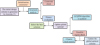 |
Fig. 3 Steps of wind-resistant optimization structural design of the large-span roof. |
3 Results
3.1 Algorithm performance comparison and convergence analysis
In large-span roof structures, 10080 members are randomly initialized into 13 categories based on the initial cross-sectional area in Table 1. [v] represents the maximum allowable deformation of the steel structure under load. [σ] is the maximum allowable stress that the component material of the steel structure can withstand under normal use. [v] = 0.206 m, and [σ] = 235MPa.  and
and  are the maximum and minimum allowable sectional area of circular steel pipes in the standard, which are 1.41 × 10² m2 and 0.76 × 10⁻² m2, respectively.
Figure 4 shows the convergence process of optimal solution design variables based on PSO algorithm.
According to Figure 4a, the first 3th dimensions variables in the PSO algorithm converged rapidly in the first 30 generations, followed by a decrease in oscillation and convergence around 140 generations. Among the variables in the 4th to 6th dimensions, the 4th and 6th dimensions converged faster in the first 30 generations and eventually converged around 180 generations, while the 5th dimension converged faster in the first 60 generations and finally converged around 130 generations. Among the 7–9 dimensional variables, the 7th and 8th dimensions converged rapidly in the first 70 generations, the 9th dimension converged faster in the first 140 generations, and ultimately all three converged before the 340 generations. Among the variables in the 10th to 13th dimensions, the 10th dimension converged faster in the first 10 generations. This convergence speed and algebraic difference are mainly due to the randomness of PSO algorithm and the complexity of large-span roof structures, especially the significant impact of wind loads on certain members. Figure 5 shows the convergence of the optimal solution variable based on QPSO.
As shown in Figure 5, the optimization calculation based on QPSO algorithm had a very fast convergence speed in the early iterations of the 1–3 dimensional variables, indicating that QPSO had strong global search ability and quickly approached the optimal solution. As the iteration progressed, the variables gradually oscillated and tended to stabilize, eventually converging around 160 generations. Compared with PSO algorithm, QPSO algorithm had a faster convergence speed, which improved the overall optimization efficiency. However, in the later stage of local search, the performance difference between the two was not significant, and both maintained the stability and accuracy. Figure 6 displays the convergence process of the optimal solution design variables on the basis of the LCQPSO.
From Figure 6, the LCQPSO algorithm had a fast convergence speed for the first 50 generations of the 1–3 dimensional variables in optimization calculations, followed by a decrease in oscillations and convergence at around 230 generations. Compared with traditional PSO and QPSO algorithms, the LCQPSO algorithm had a slightly slower convergence speed. Due to the randomness of chaotic mapping and the characteristics of chaotic local search, LCQPSO can effectively avoid getting stuck in local optima, but requires more iterations to determine the global optimum. Chaos mapping increases the complexity of the search, allowing the algorithm to explore a wider solution space and improve the quality of the final solution. Figure 7 displays the constraint variation of stress and displacement for three algorithms.
As shown in Figure 7, with the increase of iterations, the two indicators of Grey Wolf Optimizer algorithm first fluctuated greatly and then stabilized. The Whale Optimization algorithm showed a similar trend, but with slightly smaller fluctuations and faster convergence speed in the initial stage. In contrast, the LCQPSO algorithm had the smallest initial fluctuations and reached a stable state the fastest. Although the optimal particle displacement redundancy was lower than the stress redundancy, the displacement redundancy of other particles may still exceed the constraint value. Figure 8 shows the normalized constraint values of the three algorithms during the optimization process.
As shown in Figure 8, with the increase of iterations, the normalized constraint values of the three algorithms gradually decreased to 0. Figure 9 shows the particle search space mapping of three algorithms at some key iteration moments, intuitively reflecting the search behavior and optimization effects of each algorithm at different stages.
In Figure 9, at the initial iteration (t = 1), there were 4, 3, and 4 initial particles in the three algorithms on the vertical axis, respectively, which belonged to feasible solutions. At t = 40, most of the particles in the PSO were close to the vertical axis. At t = 80, PSO already had 8 particles as feasible solutions, and the particles of QPSO and LCQPSO gradually approached the vertical axis. At t = 120, all particles of PSO were feasible solutions, while QPSO and LCQPSO reached feasible solutions after 220 and 260 iterations, respectively.
Initial sectional area and number of components.
 |
Fig. 4 Design variable convergence process based on optimal solution of PSO algorithm. |
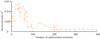 |
Fig. 5 Variable convergence of optimal solution based on QPSO. |
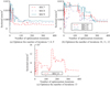 |
Fig. 6 Design variable convergence process of optimal solution based on LCQPSO algorithm. |
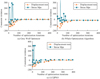 |
Fig. 7 Constraint redundancy of the three algorithms. |
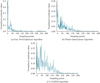 |
Fig. 8 The population constraints optimized by the three algorithms violate the mean value. |
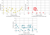 |
Fig. 9 Particle search space mapping of the three algorithms at some typical moments. |
3.2 Practical evaluation of optimization results
Figure 10 shows the performance comparison results of three algorithms.
As shown in Figure 10, LCQPSO algorithm has the best performance in the whole iteration process, and its objective function value decreases rapidly and stabilizes at a low level, and AUC value is close to 0.92, indicating that the algorithm has high optimization efficiency and stability. In contrast, although PSO and QPSO algorithms also show good convergence, they are slightly worse than LCQPSO in terms of the decline speed and stability of the objective function value. The PSO algorithm rapidly drops below 0.1 in the first 50 iterations and then tends to be stable. The QPSO algorithm decreases rapidly in the first 50 iterations, but the optimization speed slows down in 50 to 200 iterations, and becomes stable after 200 iterations. These results show that the LCQPSO algorithm with chaotic mapping can effectively improve the search efficiency and global optimization ability, especially when dealing with complex engineering optimization problems, it can find the optimal solution faster and maintain the stability of the algorithm. Figure 11 shows the mean normalization of population objective function values for three algorithms.
From Figure 11a, in the first 50 iterations of the PSO algorithm, the objective function value rapidly decreased from about 0.45 to below 0.1, demonstrating the early rapid convergence ability. After 50 iterations, the descent rate slowed down and gradually stabilized, and the fluctuation of the objective function value was small, indicating that the algorithm was conducting local search. At 150 iterations, the objective function value remained stable at a level close to 0, indicating that the PSO algorithm found the optimal solution. In Figure 11b, the QPSO algorithm had a normalized objective function value of approximately 0.5 at the initial iteration, which rapidly decreased in the first 50 iterations and exhibited a fast convergence speed. From 50 to 200 iterations, the objective function value slowly decreased, indicating that the algorithm was gradually optimizing but the speed was slowing down. After 200 iterations, the objective function value tended to be stable and close to 0, indicating that the algorithm basically converged. In Figure 11c, the LCQPSO algorithm converged rapidly in the first 50 iterations, with an obvious decrease in the objective function value. After 200 iterations, the algorithm had good stability and the objective function value tended to be stable, indicating that the algorithm found a better solution.
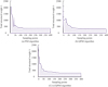 |
Fig. 10 Convergence process of objective function. |
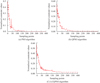 |
Fig. 11 Normalized value of overall objective function during the iteration process of three algorithms. |
4 Discussion and conclusion
To optimize the wind resistance performance and design efficiency of skyscrapers under strong wind conditions, this study introduced chaotic mapping to replace random numbers in the QPSO algorithm, and used chaotic local search technology to update the Gbest. The results indicated that in terms of stress constraints, LCQPSO reached its peak later than the other two algorithms. In terms of displacement constraints, PSO, QPSO, and LCQPSO reached their maximum violation amounts in the 10th, 44th, and 52nd generations, respectively. The three algorithms converged quickly in the initial stage, significantly reduced the total weight, and ultimately achieved the optimal solution. For the objective function value, the PSO rapidly decreased from 0.45 to below 0.1 in the first 50 generations, and stabilized after 150 generations. QPSO and LCQPSO had similar optimization efficiency in the first 200 generations, and then tended to stabilize. The chaotic mapping improved the global search capability. The optimization results show that the stress and displacement under maximum wind load meet the design requirements. wever, current research mainly focuses on specific wind direction angles and single buildings, lacking comprehensive studies on multiple buildings. In the future, the research on the comprehensive wind resistance performance of multi-building structures should be expanded, taking into account the wind load characteristics under different terrain and climate conditions. At the same time, the nonlinear characteristics of detailed structures and materials should be strengthened to improve the accuracy of simulation results. Existing algorithm models should be optimized to cope with more complex engineering application scenarios.
Funding
This research received no external funding.
Conflicts of interest
The authors have nothing to disclose.
Data availability statement
Data is provided within the manuscript.
Author contribution statement
Shifeng Wang, Conceptualization, methodology, formal analysis, supervision, writing—original draft preparation, writing—review and editing, software, validation, resources, data curation.
References
- H. Cui, H. An, M. Ma, Z. Han, S.C. Saha, Q. Liu, Experimental study on wind load and wind-induced interference effect of three high-rise buildings, J. Appl. Fluid Mech. 16, 2101–2114 (2023) [Google Scholar]
- Y. Li, P.P. Sun, A. Li, Y. Deng, Wind effect analysis of a high-rise ancient wooden tower with a particular architectural profile via wind tunnel test, Int. J. Architect. Heritage 17, 518–537 (2023) [Google Scholar]
- H. Xiong, Q. Xiong, B. Zhou, N. Abbas, Q. Kong, C. Yuan, Field vibration evaluation and dynamics estimation of a super high-rise building under typhoon conditions: data-model dual driven, J. Civil Struct. Health Monitor. 13, 235–249 (2023) [Google Scholar]
- A. Williams, Human-centric functional computing as an approach to human-like computation, Artif. Intell. Appl. 1, 118–137 (2023) [Google Scholar]
- N. Kumar, O. Prakash, Analysis of wind energy resources from high rise building for micro wind turbine: a review, Wind Eng. 47, 190–219 (2023) [Google Scholar]
- Q. Wang, B. Zhang, Wind-induced responses and wind loads on a super high-rise building with various cross-sections and high side ratio—a case study, Buildings 13, 485–485 (2023) [Google Scholar]
- C. Lu, Z. Yang, L. Zheng, Z. Liu, Smart reliability analysis of wind resistance of lightweight steel structures in super tall buildings in a smart city, J. Test. Evaluat. 51, 1793–1803 (2023) [Google Scholar]
- H. Cui, H. An, M. Ma, Z. Han, S.C. Saha, Q. Liu, Experimental study on wind load and wind-induced interference effect of three high-rise buildings, J. Appl. Fluid Mech. 16, 2101–2114 (2023) [Google Scholar]
- W. Sun, X. Wang, D. Dong, M. Zhang, Q. Li, A comprehensive review on estimation of equivalent static wind loads on long-span roofs, Adv. Struct. Eng. 26, 2572–2599 (2023) [Google Scholar]
- Z. Chen, C. Wei, Z. Li, C. Zeng, J. Zhao, N. Hong, N. Su, Wind-induced response characteristics and equivalent static wind-resistant design method of spherical inflatable membrane structures, Buildings 12, 1611–1611 (2022) [Google Scholar]
- Y. Liu, Y. Ru, F. Li, L. Zheng, J. Zhang, X. Chen, S. Liang, Structural design and optimization of separated air-rib tents based on response surface methodology, Appl. Sci. 13, 55–67 (2022) [Google Scholar]
- L. Wang, T. Wei, W. Zhang, J. Xiao, Design and construction of a large-span integrally tensioned structure with ETFE roof, in Proceedings of IASS Annual Symposia. International Association for Shell and Spatial Structures (IASS), 2022, 1–11 (2022) [Google Scholar]
- J. Chen, Y. Wang, K. Chen, S. Huang, X. Xu, Analyzing the form-finding of a large-span transversely stiffened suspended cable system: a method considering construction processes, World J. Eng. Technol. 12, 229–244 (2024) [Google Scholar]
- D. Zhao, Z. Yang, X. Zeng, J. Yu, Y. Gao, G. Huang, Wind tunnel test of gust load alleviation for a large-scale full aircraft model, Chin. J. Aeronaut. 36, 201–216 (2023) [Google Scholar]
- Y. Lu, J. Li, K. Yang, A hybrid calculation method of electromagnetic vibration for electrical machines considering high-frequency current harmonics, IEEE Trans. Ind. Electr. 69, 10385–10395 (2022) [Google Scholar]
- W. Sun, X. Wang, D. Dong, M. Zhang, Q. Li, A comprehensive review on estimation of equivalent static wind loads on long-span roofs, Adv. Struct. Eng. 26, 2572–2599 (2023) [Google Scholar]
- Z. Deng, B. Zhang, Y. Miao, B. Zhao, Q. Wang, K. Zhang, Multi-objective optimal design of the wind-wave hybrid platform with the coupling interaction, J. Ocean Univ. China 22, 1165–1180 (2023) [Google Scholar]
- X. Liu, G.G. Wang, L. Wang, LSFQPSO: quantum particle swarm optimization with optimal guided Lévy flight and straight flight for solving optimization problems, Eng. Comput. 38, 4651–4682 (2022) [Google Scholar]
- M. Alawida, J.S. Teh, A. Mehmood, A. Shoufan, A chaos-based block cipher based on an enhanced logistic map and simultaneous confusion-diffusion operations, J. King Saud Univ. Comput. Inf. Sci. 34, 8136–8151 (2022) [Google Scholar]
- H. Pradhan, B.B. Mangaraj, S.K. Behera, Chebyshev-based array for beam steering and null positioning using modified ant lion optimization, Int. J. Microwave Wireless Technolog. 14, 143–157 (2022) [Google Scholar]
Cite this article as: S. Wang: Wind resistance performance optimization of PSO algorithm in skyscrapers design. Sust. Build. 8, 2 (2025), https://doi.org/10.1051/sbuild/2025002.
All Tables
All Figures
|
Fig. 1 Definition of test wind direction and arrangement of measuring points. |
| In the text | |
|
Fig. 2 Wind resistance optimization process of super tall building structure based on QPSO algorithm. |
| In the text | |
|
Fig. 3 Steps of wind-resistant optimization structural design of the large-span roof. |
| In the text | |
|
Fig. 4 Design variable convergence process based on optimal solution of PSO algorithm. |
| In the text | |
|
Fig. 5 Variable convergence of optimal solution based on QPSO. |
| In the text | |
|
Fig. 6 Design variable convergence process of optimal solution based on LCQPSO algorithm. |
| In the text | |
|
Fig. 7 Constraint redundancy of the three algorithms. |
| In the text | |
|
Fig. 8 The population constraints optimized by the three algorithms violate the mean value. |
| In the text | |
|
Fig. 9 Particle search space mapping of the three algorithms at some typical moments. |
| In the text | |
|
Fig. 10 Convergence process of objective function. |
| In the text | |
|
Fig. 11 Normalized value of overall objective function during the iteration process of three algorithms. |
| In the text | |
Current usage metrics show cumulative count of Article Views (full-text article views including HTML views, PDF and ePub downloads, according to the available data) and Abstracts Views on Vision4Press platform.
Data correspond to usage on the plateform after 2015. The current usage metrics is available 48-96 hours after online publication and is updated daily on week days.
Initial download of the metrics may take a while.